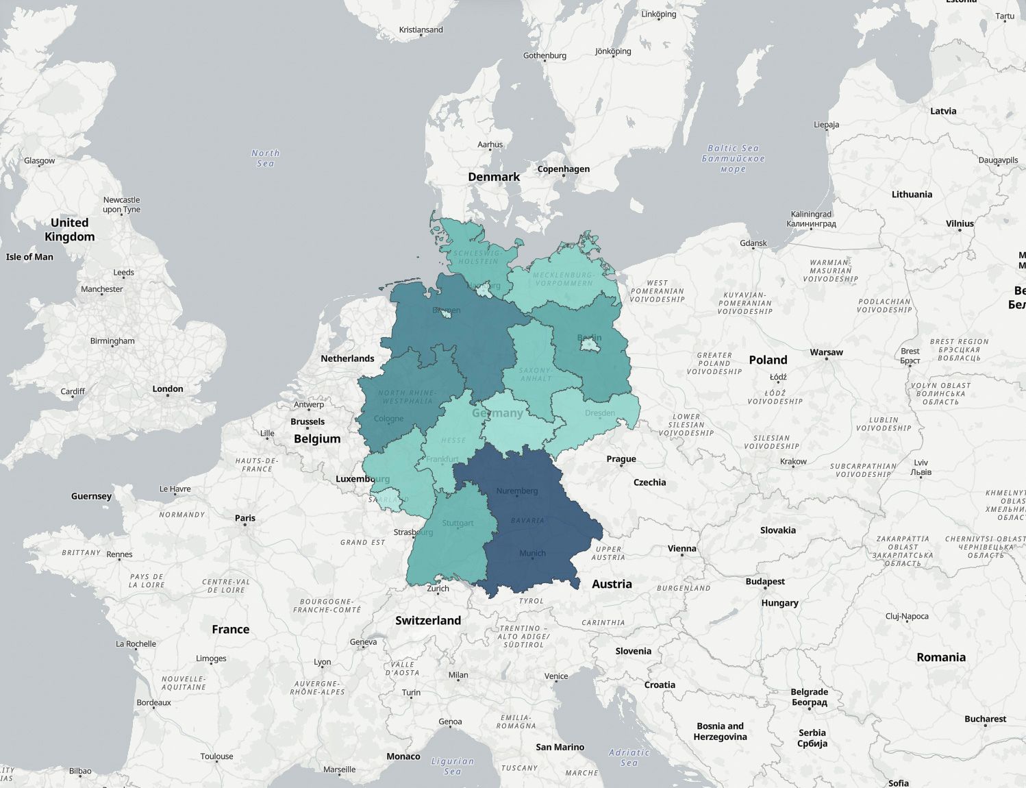
At its core, Energy Workbench is the quantitative engine behind our own projects – the same data and models our analysts open every day. What you see on the platform is a live preview of what that engine can do.
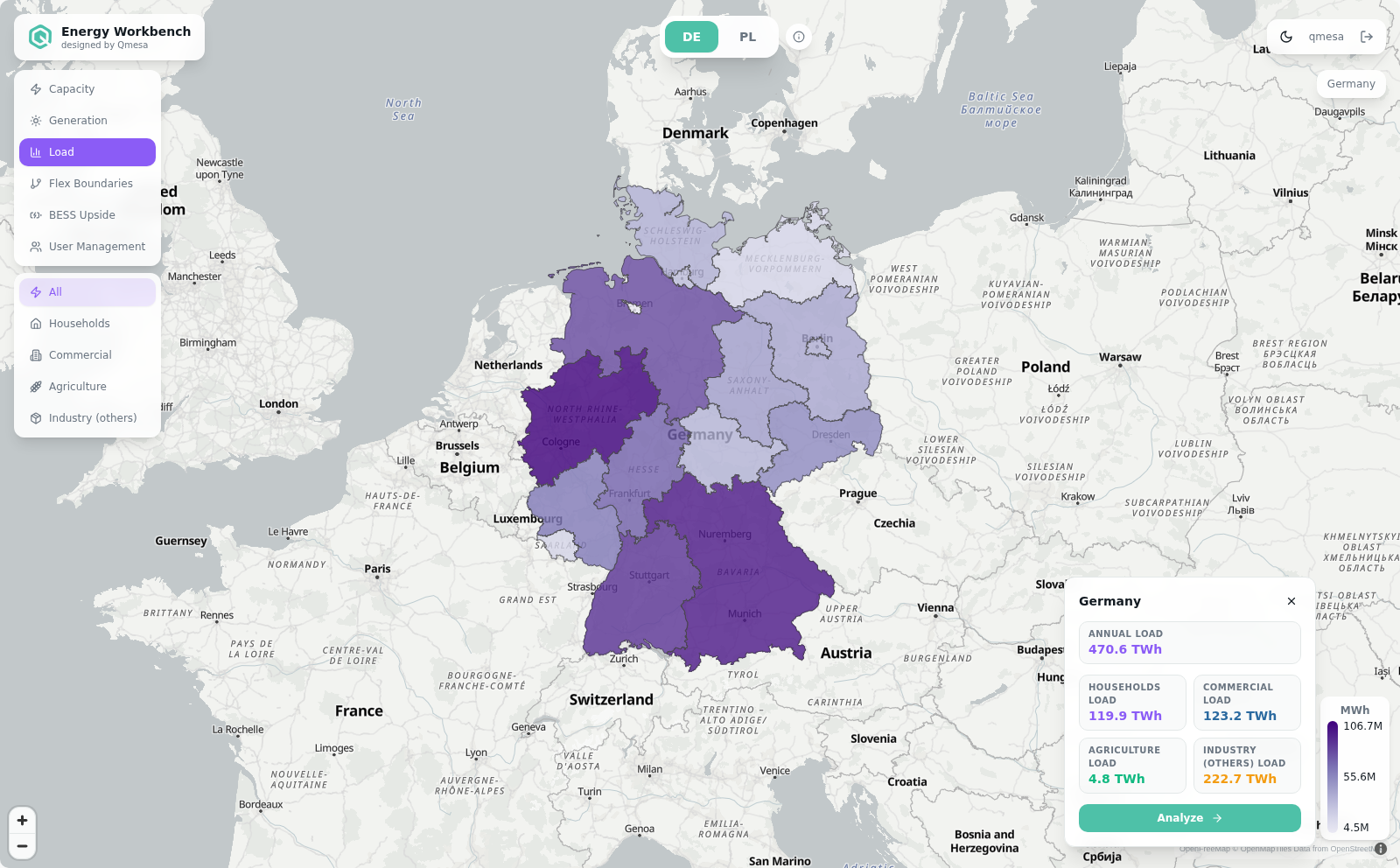
The hard part isn't the map. It's making the analysis underneath it defensible. A MaStR or URE register gives you installed capacity; getting from there to an hourly production profile takes a weather-driven model. National statistics give you total demand; putting it on the map takes a spatial and sectoral split. Flexible-connection boundaries follow from regional net load. And a revenue comparison is only ever as good as the dispatch logic behind it.
So we built the platform as one connected chain, each module feeding the next. Registered capacity (PV and wind, down to the municipality) feeds a weather-driven generation profile. Generation meets modelled load to give regional net load – the local surplus or deficit that actually drives flexibility value. And net load sets the flex boundaries: how much a battery can charge or discharge each hour while staying inside the local grid's limits.
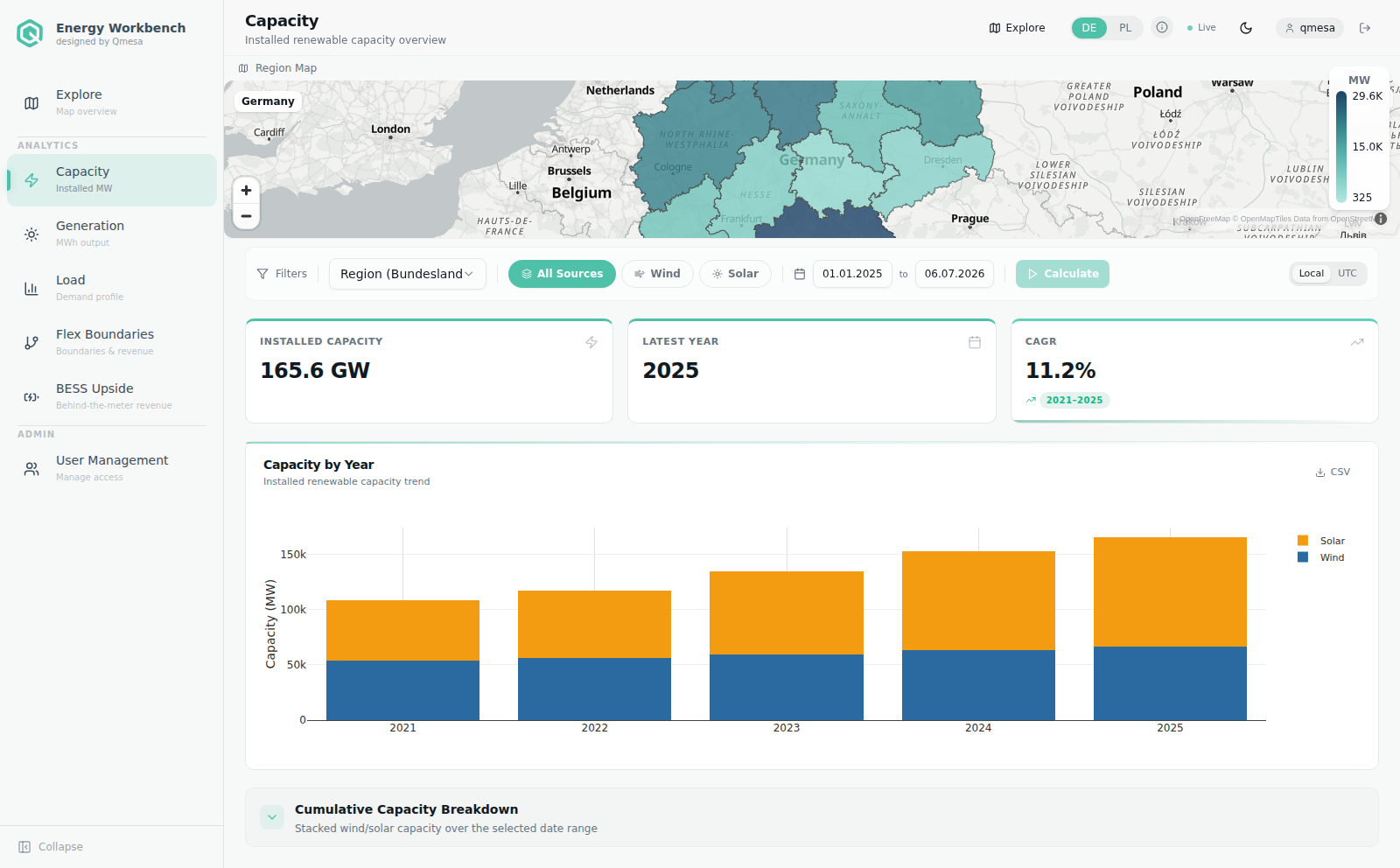
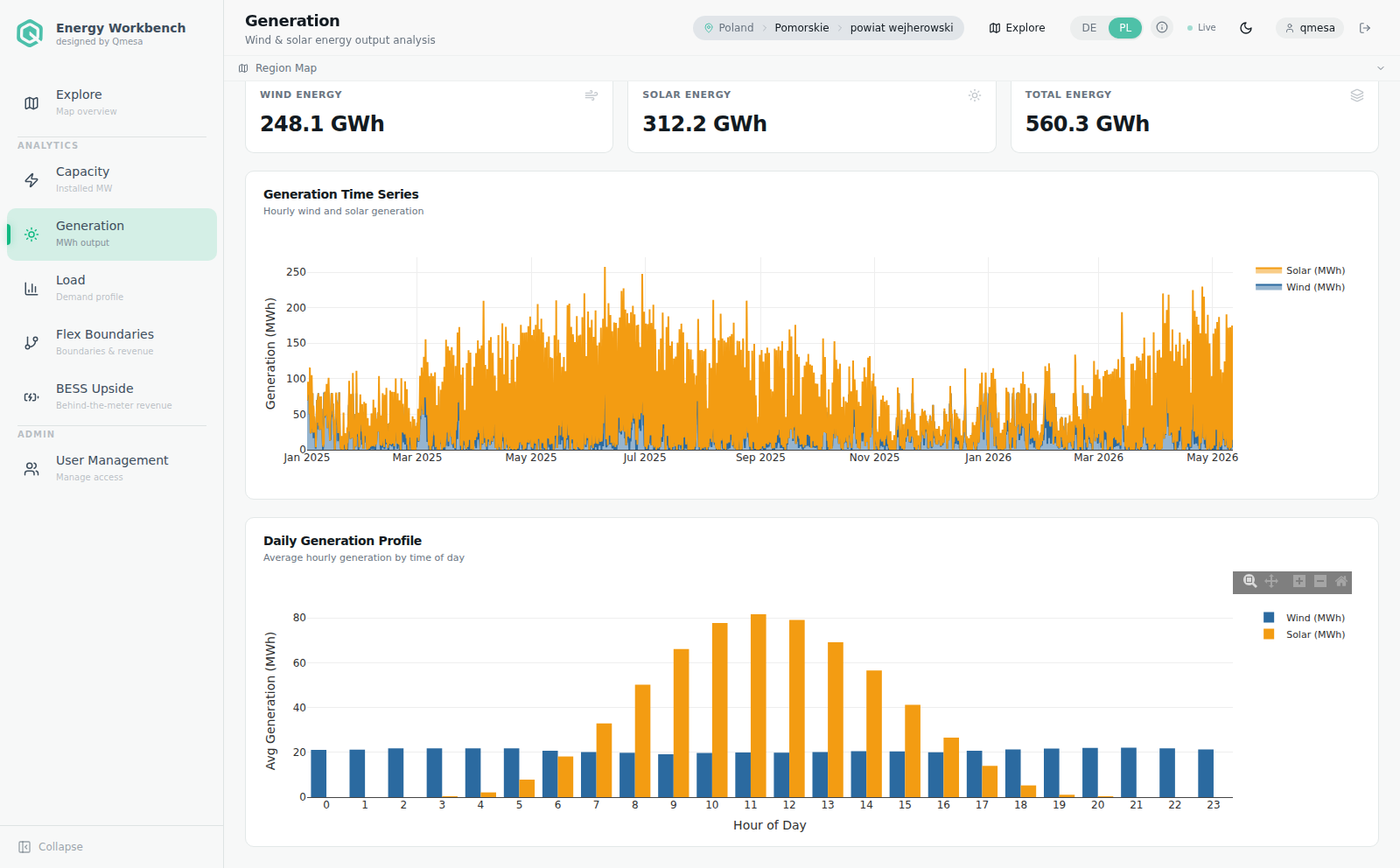
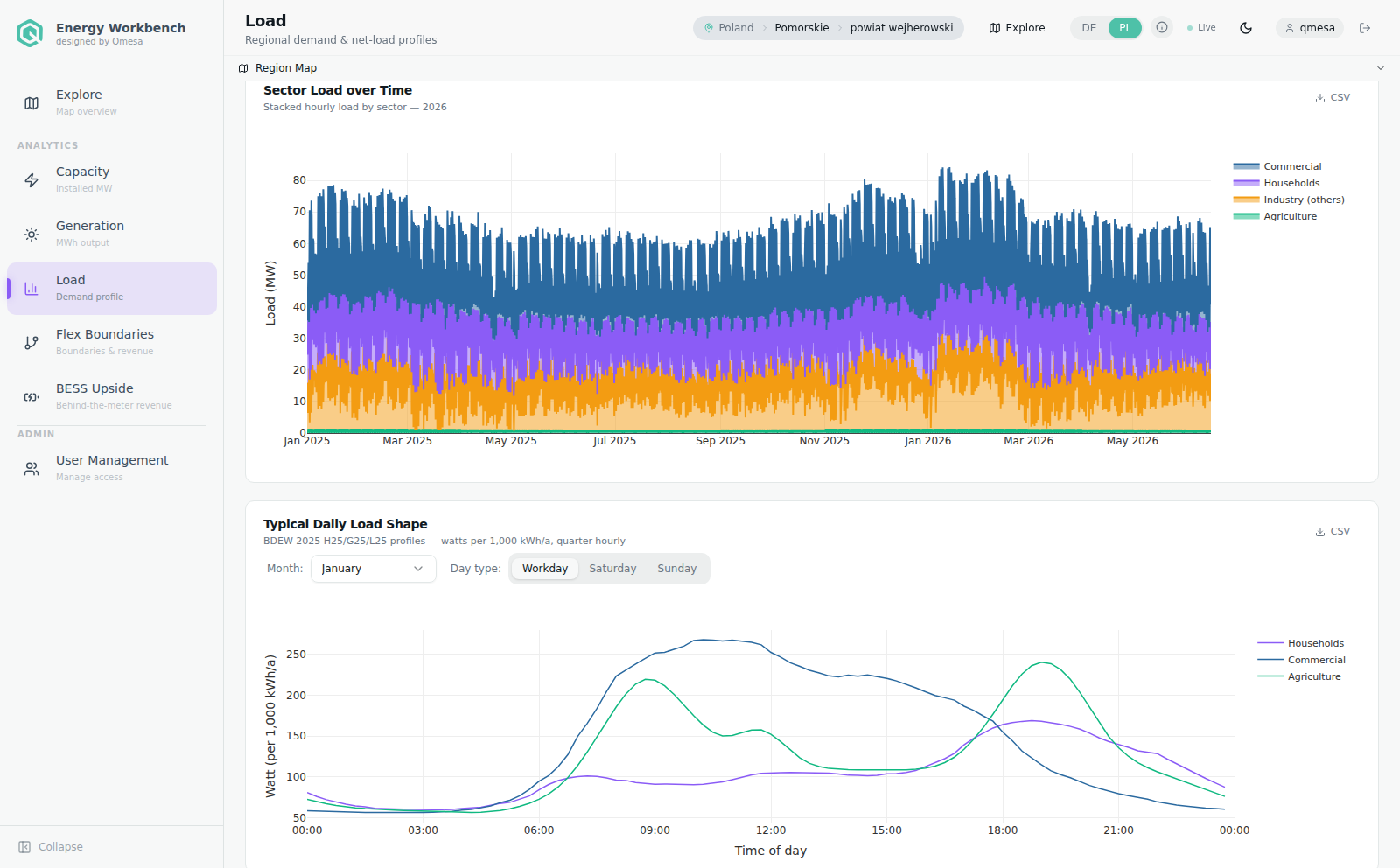
Take load, the middle of that chain. Where does demand actually sit? Energy Workbench shows it down to the municipality: high-granularity electricity demand, built from JRC population and built-up rasters, split by sector into households, commercial, agriculture and industry (others), and shaped quarter-hour by quarter-hour with BDEW standard load profiles – all reconciled against measured ENTSO-E national load and Eurostat sector balances. Put that demand next to local RES generation and you start to see where a BESS earns more, well before you commit to a connection point.
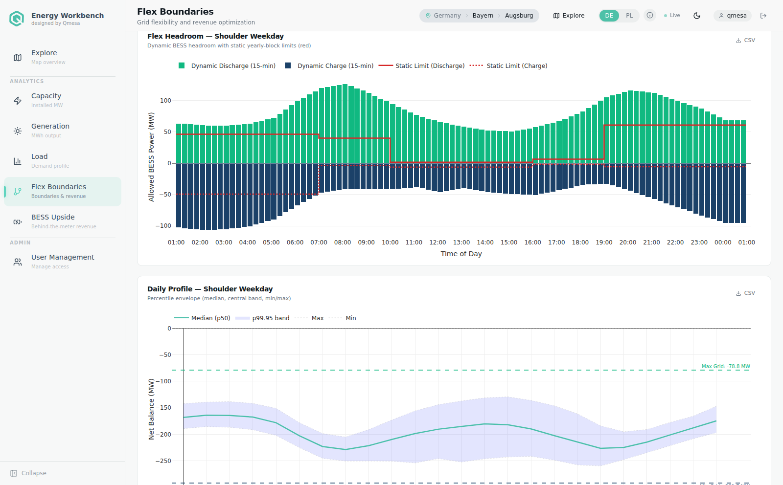
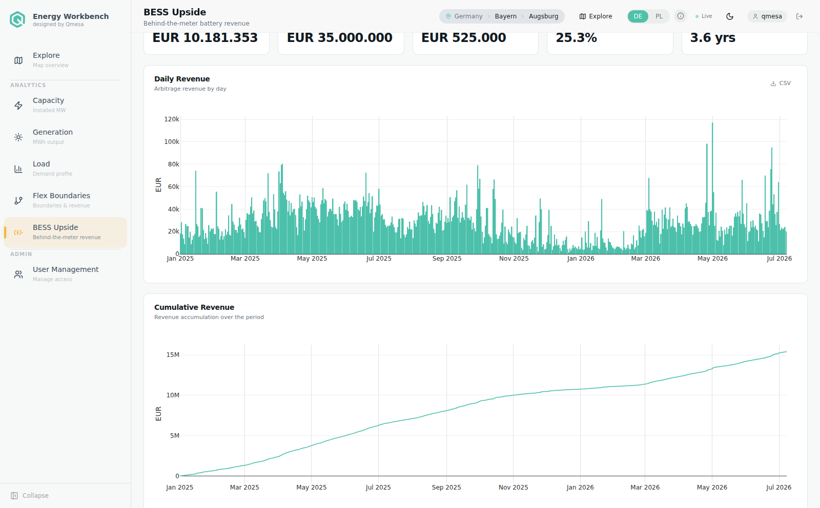
On top of that net load, the flex module values the battery against real constraints, using actual day-ahead prices: grid-neutral flex boundaries, a static year-round envelope, and – for a behind-the-meter asset – discharge capped at on-site load (BESS Upside). Each run comes with IRR and payback, so the cost of a connection or self-consumption constraint shows up as a number you can read straight off the screen.
Energy Workbench is AaaS: Analytics as a Service. The free features are built for comparison and benchmarking – flex vs. static IRR, your project assumptions against the regional reference. Want to go deeper? Personalised access focuses the same analytical layer on your own portfolio and questions.
Think of it as an analytical layer offered as a service: the engine behind our advisory work, made faster and more transparent for you.
Access is free, and both Polish and German data are live today.
1. Open Energy Workbench and choose Request access on the sign-in panel.
2. Enter your work email. That's all we ask for.
3. We review the request and send your login by email.
Prefer email? Write to workbench@qmesa.eu and we'll set you up.
